Population mean size-at-age (LAA)
1. Parametric LAA
For \(y=1\) at the start of the year (Richards 1959):
\[
\tilde{L}_{y,a} = \begin{cases}
L'_{min} + ba,\hspace{6cm}a\leq \tilde{a}\\
(L_\infty^\gamma + (L_\tilde{a}^\gamma-L_\infty^\gamma)exp(-k(a-\tilde{a})))^{1/\gamma}\hspace{1cm}a>\tilde{a}
\end{cases}
\]
Where \(L'_{min}\) is the lower limit of the smallest length bin, \(\tilde{a}\) is the reference age, \(L_\infty\) is the asymptotic length, \(k\) is the growth rate, \(\gamma\) is the shape parameter. Also, \(b=(L_\tilde{a} - L'_{min})/\tilde{a}\).
1. Parametric LAA
For \(y>1\):
\[
\tilde{L}_{y,a} = \begin{cases}
L'_{min} + ba,\hspace{7cm}a\leq \tilde{a}\\
(\tilde{L}_{y-1,a-1}^\gamma + (\tilde{L}_{y-1,a-1}^\gamma-L_\infty^\gamma)(exp(-k)-1))^{1/\gamma}\hspace{0.5cm}a>\tilde{a}
\end{cases}
\]
When \(\gamma = 1\), the equation is von Bertalanffy (Schnute 1981).
1. Parametric LAA
For any fraction \(\theta\) of the year:
\[\tilde{L}_{y,a+\theta}=(\tilde{L}_{y-1,a-1}^\gamma + (\tilde{L}^\gamma_{y-1,a-1})(exp(-k\theta)-1))^{1/\gamma}\]
This is particularly important since fish also grow within a year.
1. Parametric LAA
To model time-variability, we could predict deviations on any growth parameter:
\[log(P_t) = \mu_P + \delta_{P,t}\]
Where \(P\) represents the growth parameter, and \(t\) represents years or cohorts.
The structure of these deviations \(\delta_{P,t}\) could be independent or correlated over time.
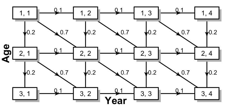
2. Nonparametric LAA
Input population mean size-at-age \(\tilde{L}_{a}\) are treated as fixed effects. We do not need any kind of parametric equation. If time-invariant growth, so \(\tilde{L}_{a,y}=\tilde{L}_{a}\) for all \(y\).
To model growth within a year, we use a linear interpolation between \(\tilde{L}_{a,y}\) and \(\tilde{L}_{a+1,y+1}\).
2. Nonparametric LAA
If we want to model time-varying growth, we predict deviations:
\[\tilde{L}_{a,y} = \mu_{\tilde{L}_{a}} + \delta_{a,y}\]
Where the structure of these deviations \(\delta_{a,y}\) could be independent or correlated over time and ages, or correlated over ages, years, and cohorts (Cheng et al. 2023).
2. Nonparametric LAA
Deviations structure (correlation over years and ages):
\[E \sim MVN(0, \Sigma)\]
\(E = (\varepsilon_{1,1},...,\varepsilon_{1,Y-1},\varepsilon_{2,1},...,\varepsilon_{1,Y-1},...,\varepsilon_{A,1},...,\varepsilon_{A,Y-1})'\), \(Y\) is the number of years, and \(\Sigma\) is the covariance matrix:
\[Cov(\varepsilon_{a,y},\tilde{\varepsilon}_{a,y}) = \frac{\sigma_G\rho_{a}^{\vert a-\tilde{a} \vert}\rho_{y}^{\vert y-\tilde{y} \vert}}{(1-\rho^2_a)(1-\rho_y^2)}\]
where \(-1<\rho_a <1\) and \(-1<\rho_y <1\) are the autocorrelation coefficients (fixed effects).
2. Nonparametric LAA
We could also estimate partial autocorrelation coefficients by year, age and cohorts (Cheng et al. 2023).
![]()
3. Semiparametric LAA
Only used to model time-varying growth. It is a combination of the previous two approaches. We follow these steps:
We calculate the population mean size-at-age at the start of the year using a parametric equation (e.g., von Bertalanffy).
Predict deviations from the values calculated in the previous step. Structure could be independent or correlated over time and ages.
Calculate population mean size-at-age within a year using linear interpolation.
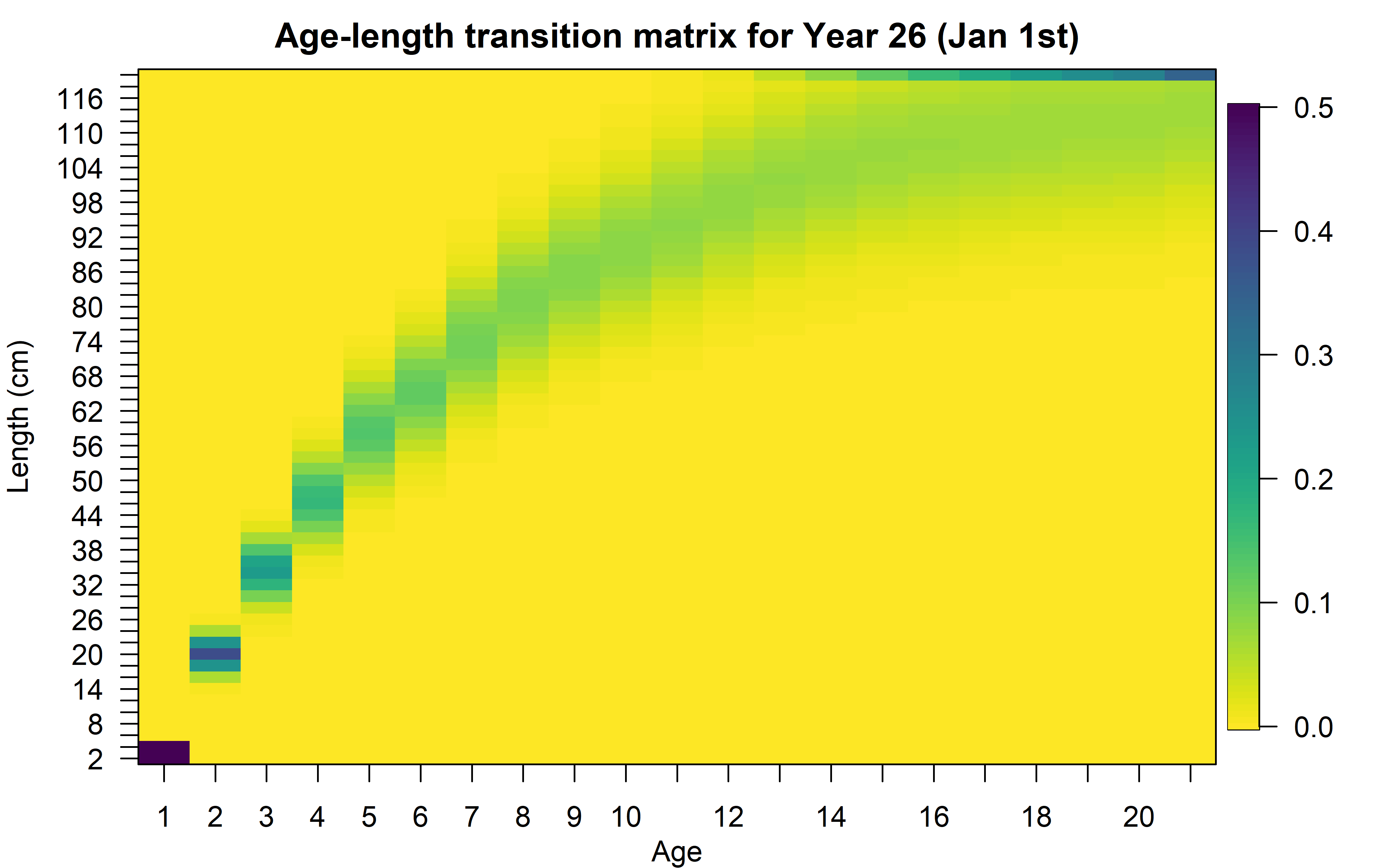
Transition matrix
Distribute the information of each age among length bins:
\[\varphi_{y,l,a}=\begin{cases}
\Phi(\frac{L'_{min^\ast} - L_{y,a}}{\sigma_{y,a}})\hspace{3.2cm}l=1\\
\Phi(\frac{L'_{l+1} - L_{y,a}}{\sigma_{y,a}})-\Phi(\frac{L'_{l} - L_{y,a}}{\sigma_{y,a}})\hspace{1cm}1<l<n_L\\
1-\Phi(\frac{L'_{max} - L_{y,a}}{\sigma_{y,a}})\hspace{2.5cm}l=n_L
\end{cases}\]
\(\Phi\) is the cumulative standard normal distribution, \(L'_{min^\ast}\) is the smallest length bin, \(l\) is the length bin index, \(n_L\) is the number of length bins, and \(\sigma_{y,a}\) is the standard deviation of lengths for age \(a\).
Transition matrix
\(\sigma_{y,a}\) is calculated from two parameters: \(\sigma_{\tilde{a}}\) y \(\sigma_{A}\):
\[\sigma_{y,a}=\sigma_{\tilde{a}}+(\frac{\sigma_{A}-\sigma_{\tilde{a}}}{L_{\infty}-L_{\tilde{a}}})(\tilde{L}_{y,a}-L_{\tilde{a}})\]
For the nonparametric LAA approach, we use \(L_A\) instead of \(L_{\infty}\) and \(L_1\) instead of \(L_{\tilde{a}}\).
Transition matrix
![]()
Population mean weight-at-age (WAA)
1. Parametric WAA
When we model the population mean size-at-age, we can use the length-weight relationship:
\[W_{l} = \Omega_1 {L_l}^{\Omega_2}\]
Where \(\Omega_1\) and \(\Omega_2\) are parameters (fixed effects).
We could also model time-varying L-W parameters (independent or correlated over time).
1. Parametric WAA
Then, to calculate the population mean weight-at-age:
\[W_{y,a}=\sum_l \varphi_{y,l,a}W_{l}\]
2. Nonparametric WAA
Same approach as described for the nonparametric LAA.
We have a vector of population mean weight-at-age \(\tilde{W}_{a}\) at the start of a year, treated as fixed effects. For time-invariant growth, then \(\tilde{W}_{a,y}=\tilde{W}_{a}\) for every \(y\).
The mean weight-at-age within a year is calculated as:
\[\tilde{W}_{y,a+\theta} = \tilde{W}_{y,a}(G_{y,a})^\theta\]
Where \(G_{y,a} = \tilde{W}_{y+1,a+1}/\tilde{W}_{y,a}\).
2. Nonparametric WAA
To model temporal variability, we can predict deviations:
\[\tilde{W}_{a,y} = \mu_{\tilde{W}_{a}} + \delta_{a,y}\]
Where these deviations \(\delta_{a,y}\) can be independent or correlated over time and ages, or correlated over time, ages, and cohorts.
Expected catch-at-age and length
We use:
\[\hat{C}_{y,f,l,a} = \varphi_{y,l,a}S_{y,f,l}S_{y,f,a}F_{y,f}N_{y,a}\frac{1-exp(-Z_{y,a})}{Z_{y,a}}\]
Where \(f\) represents the fisheries and \(Z_{y,a}\) is calculated using aggregated \(F\) and selectivity-at-age.
Age and length compositions
First, we sum over ages or lengths:
\[\hat{C}_{y,f,a} = \sum_l{\hat{C}_{y,f,l,a}}\hspace{2cm}\hat{C}_{y,f,l} = \sum_a{\hat{C}_{y,f,l,a}}\]
Then, we calculate the marginal composition (proportions):
\[\hat{p}_{y,f,a}=\frac{\hat{C}_{y,f,a}}{\sum_{a}\hat{C}_{y,f,a}}\hspace{2cm}\hat{p}_{y,f,l}=\frac{\hat{C}_{y,f,l}}{\sum_{l}\hat{C}_{y,f,l}}\]
Aggregated catch
We calculate:
\[\hat{C}_{y,f}=\sum_a W_{y,a}\hat{C}_{y,f,a}\]
Where \(W_{y,a}\) is the population mean weight-at-age that corresponds to the fishery \(f\) (year fraction).
Index of abundance
We calculate:
\[\hat{I}_{y,i,l,a}=\varphi_{y,l,a}S_{y,i,l}S_{y,i,a}N_{a,y}exp(-f_{y,i}Z_{a,y})\]
Where \(i\) is the index of abundance and \(f_{y,i}\) is the year fraction when the survey takes place.
Index of abundance
We then calculate the summation over ages or lengths:
\[\hat{I}_{y,i,a} = \sum_l{\hat{I}_{y,i,l,a}}\hspace{2cm}\hat{I}_{y,i,l} = \sum_a{\hat{I}_{y,i,l,a}}\]
Then, we calculate the marginal composition (proportion):
\[\hat{p}_{y,i,a}=\frac{\hat{I}_{y,i,a}}{\sum_{a}\hat{I}_{y,i,a}}\hspace{2cm}\hat{p}_{y,i,l}=\frac{\hat{I}_{y,i,l}}{\sum_{l}\hat{I}_{y,i,l}}\]
Index of abundance
The aggregated index value (in weight):
\[\hat{I}_{y,i} = Q_{y,i}\sum_a W_{y,a}\hat{I}_{y,i,a}\]
Where \(Q\) is the catchability and \(W_{y,a}\) is the population weight-at-age that corresponds to that index.
For the index value in numbers, we simply omit \(W_{y,a}\).
 Modeling time-varying growth in WHAM