Accounting for temporal variability in somatic growth improves a state-space assessment model for walleye pollock in the Gulf of Alaska
Giancarlo M. Correa\(^1\), Cole Monnahan\(^2\), Jane Sullivan\(^3\), James T. Thorson\(^2\), Andre E. Punt\(^1\)
\(^1\)University of Washington, Seattle, WA
\(^2\)Alaska Fisheries Science Center, NOAA, Seattle, WA
\(^3\)Alaska Fisheries Science Center, NOAA, Juneau, AK
The Woods Hole Assessment Model (WHAM)
- Fully state-space age-structured model
- Data: catch, indices of abundance, age compositions, empirical weight-at-age, environmental covariates
- Separability of total catch and proportions-at-age, as well as annual F and selectivity
- Random effects in selectivity, M, NAA, Q
- Written in TMB and R (user friendly!) ( see R package ).
Stock and Miller (2021)
The Woods Hole Assessment Model (WHAM)
Limitations:
- Lack of best practices for random effects use
- growth cannot be modeled internally
- selectivity-at-age options but not selectivity-at-length
- single sex, no spatial component, no aging error
WHAM expansion
Data inputs
- (Marginal) length compositions
- Conditional age-at-length
Growth modeling
Growth modeling overview
In the population:
Mean length-at-age (LAA)
Growth equation (von Bertalanffy)
The mean length-at-age at the start of the year (\(y=1\)):
\[\tilde{L}_{y,a} = L_{\infty}+(L_1 - L_{\infty})exp(-k(a-1))\]
\(a=1\) is first age in WHAM. Then, when \(y>1\):
\[\tilde{L}_{y,a} = \begin{cases} L_1, & \mbox{if } a=1 \\ \tilde{L}_{y-1,a-1}+(\tilde{L}_{y-1,a-1}-L_{\infty})(exp(-k)-1) & \mbox{otherwise} \end{cases}\]
Mean length-at-age (LAA)
Growth equation (von Bertalanffy)
Then, to calculate the mean length-at-age at any fraction of the year:
\[L_{y,a} = \tilde{L}_{y,a} + (\tilde{L}_{y,a} - L_{\infty})(exp(-kf_y)-1)\] \(f_y\) is the year fraction.
Mean length-at-age (LAA)
Growth equation (von Bertalanffy)
Also, \(L_{y,a}\) and variation of length-at-age ( \(\sigma_{y,a}\) ) are used to calculate the age-length transition matrix (Stock Synthesis - SS - approach):
\[\varphi_{y,l,a} = \begin{cases} \Phi(\frac{L'_{min}-L_{y,a}}{\sigma_{y,a}}) & \mbox{for } l=1 \\ \Phi(\frac{L'_{l+1} - L_{y,a}}{\sigma_{y,a}}) - \Phi(\frac{L'_{l} - L_{y,a}}{\sigma_{y,a}}) & \mbox{for } 1<l<n_L \\ 1-\Phi(\frac{L'_{max} - L_{y,a}}{\sigma_{y,a}}) & \mbox{for } l = n_L \end{cases}\]
Where \(\Phi\) is standard normal cumulative density function, \(L'_{l}\) is the lower limit of length bin \(l\), \(L'_{min}\) is the upper limit of the smallest length bin, \(L'_{max}\) is the lower limit of the largest length bin, and \(n_L\) is the largest length bin index.
Mean length-at-age (LAA)
Growth equation (von Bertalanffy)
Random effects on growth parameters can be predicted (notice log scale):
\[log(L_{\infty_t}) = \mu_{L_\infty} + \delta_{1,t}\]
\[log(k_t) = \mu_{k} + \delta_{2,t}\]
\[log(L_{1_t}) = \mu_{L_1} + \delta_{3,t}\]
\(t\) represents year or cohort effects and can be \(iid\) or \(AR1\).
Mean length-at-age (LAA)
LAA random effects
For this case, mean length-at-age ( \(\mu_{\tilde{L}_{a}}\), notice log scale ) are assumed to be parameters and can be estimated. \(\sigma_{y,a}\) still needed.
Time variability can be modeled by predicting random effects:
\[log(\tilde{L}_{y,a}) = \mu_{\tilde{L}_{a}} + \delta_{y,a}\]
\(\delta_{y,a}\) can be \(iid\) or \(2dAR1\) (full variance-covariance matrix).
Mean weight-at-age (WAA)
Length-weight relationship
Optional when empirical weight-at-age not provided:
\[w_l = \Omega_1 l^{\Omega_2}\]
Random effects on \(\Omega_1\) and \(\Omega_2\) can also be predicted.
Then:
\[\hat{w}_{y,a} = \sum_l \varphi_{y,l,a}w_l\]
\(\hat{w}_{y,a}\) can also be fitted to \(w_{y,a}\) (observed mean weight-at-age)
Mean weight-at-age (WAA)
WAA random effects
Like the LAA random effects. Mean weight-at-age ( \(\mu_{\tilde{W}_{a}}\), notice log scale ) are assumed to be parameters and can be estimated.
Time variability can be modeled by predicting random effects:
\[log(\tilde{W}_{y,a}) = \mu_{\tilde{W}_{a}} + \delta_{y,a}\]
\(\delta_{y,a}\) can be \(iid\) or \(2dAR1\) (full variance-covariance matrix).
Walleye pollock in the Gulf of Alaska (GOA)
Model overview
Data:
- One fishery (1970 to 2021) and six surveys
- Age compositions for fishery and surveys
- Mean weight-at-age for fishery and surveys
Parameters (penalized ML for time-varying quantities):
- Time-varying fishery age selectivity
- Two Qs vary over time
- Recruitment variability
Starting model
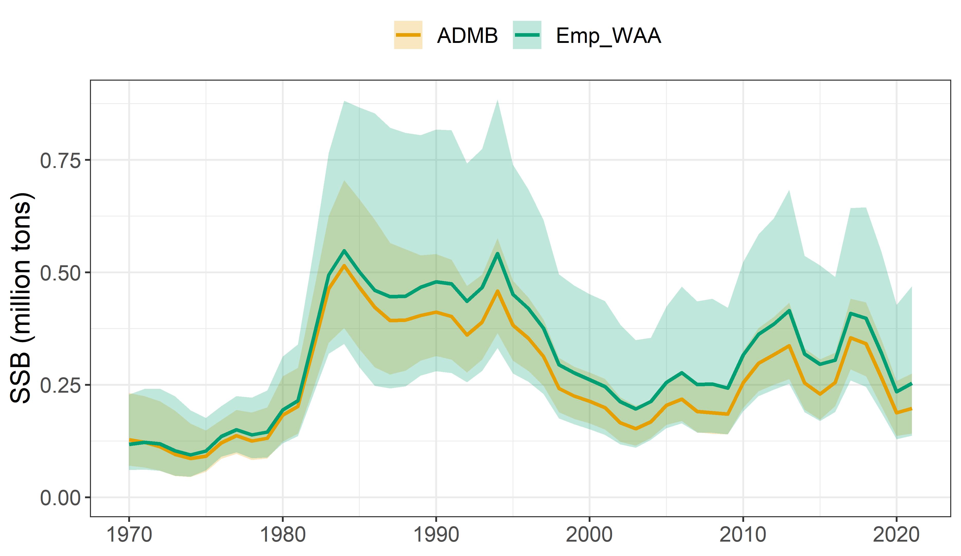
ADMB model vs WHAM model
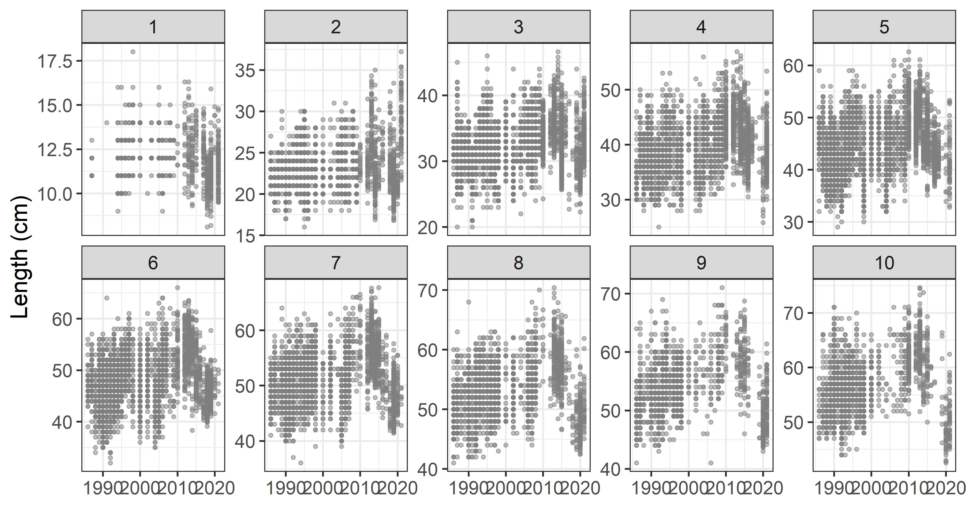
Growth variability
Observed survey fish lengths:
Growth modeling strategies
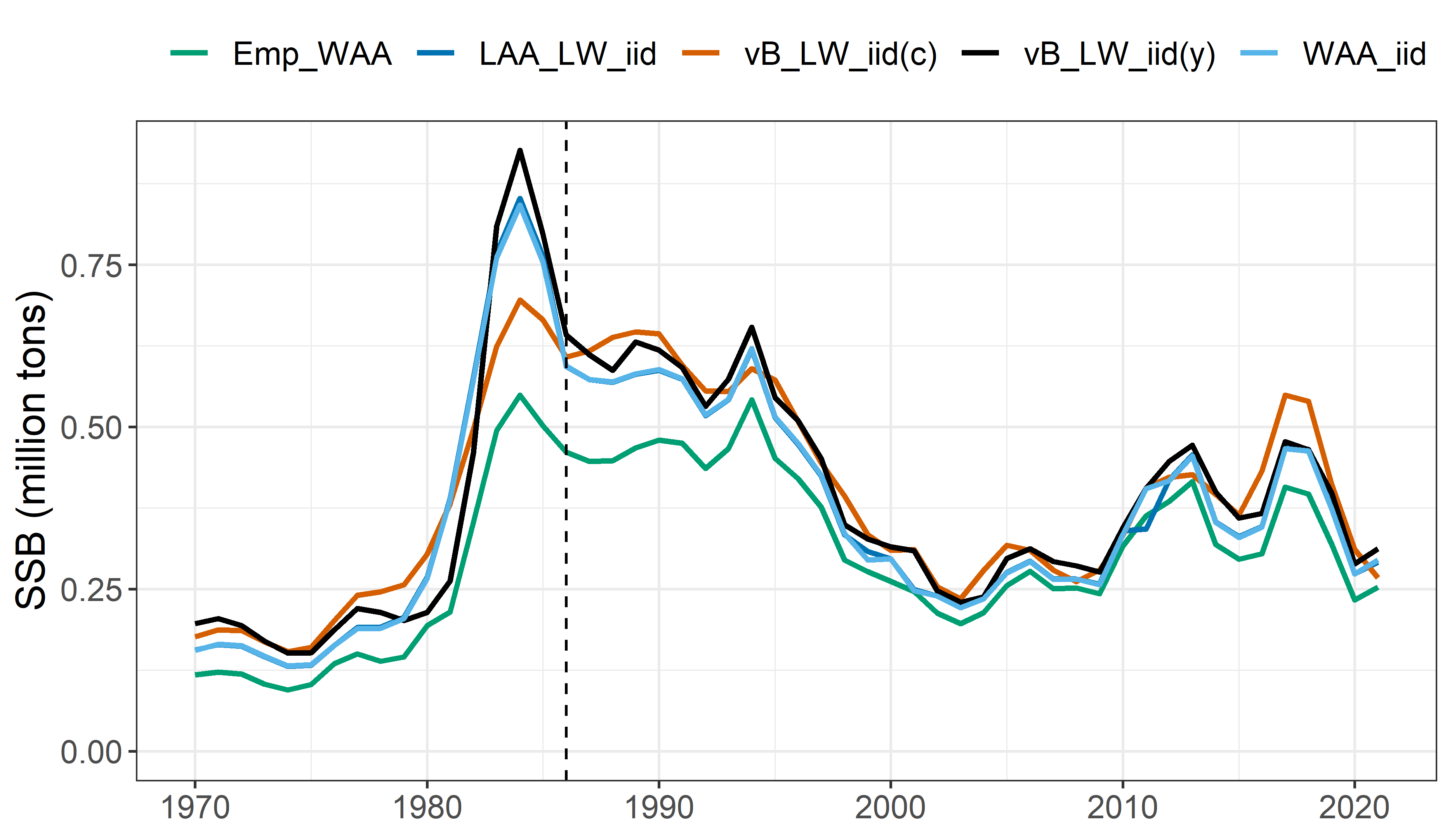
Model comparison
Mean SSB estimates:
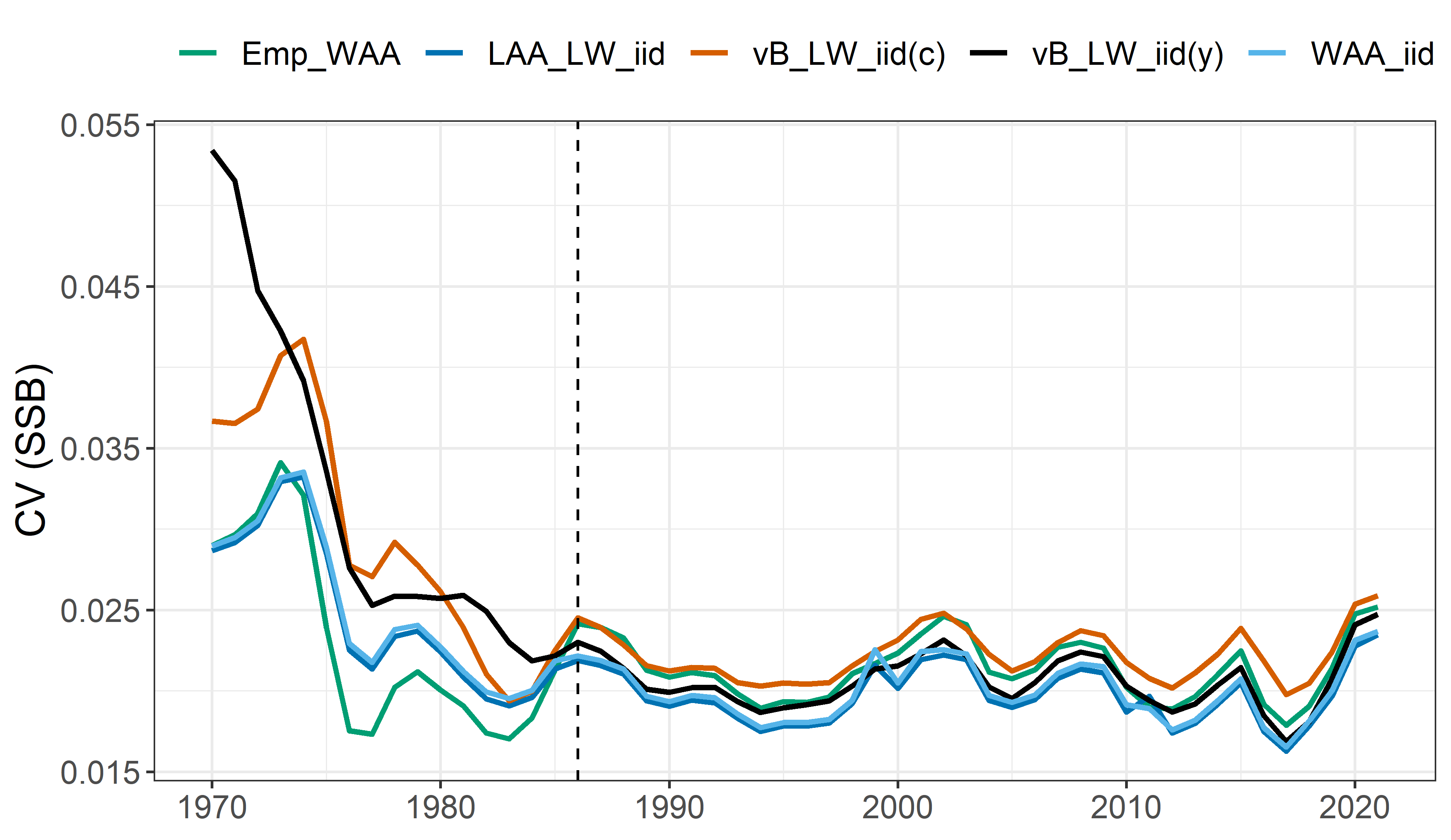
Model comparison
SSB coefficient of variation:
Model comparison
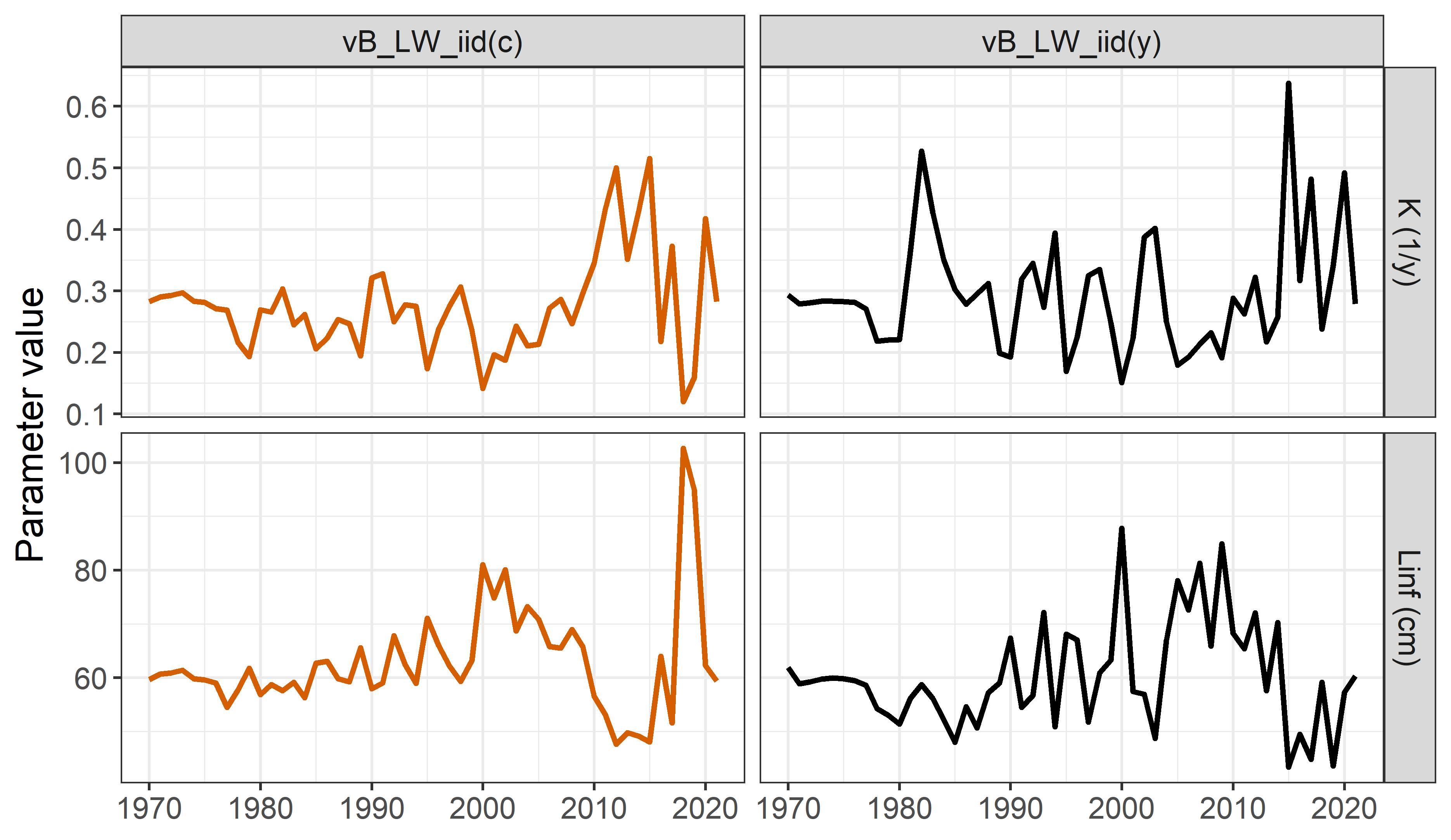
Growth parameters (only for growth parametric approach):
Model comparison
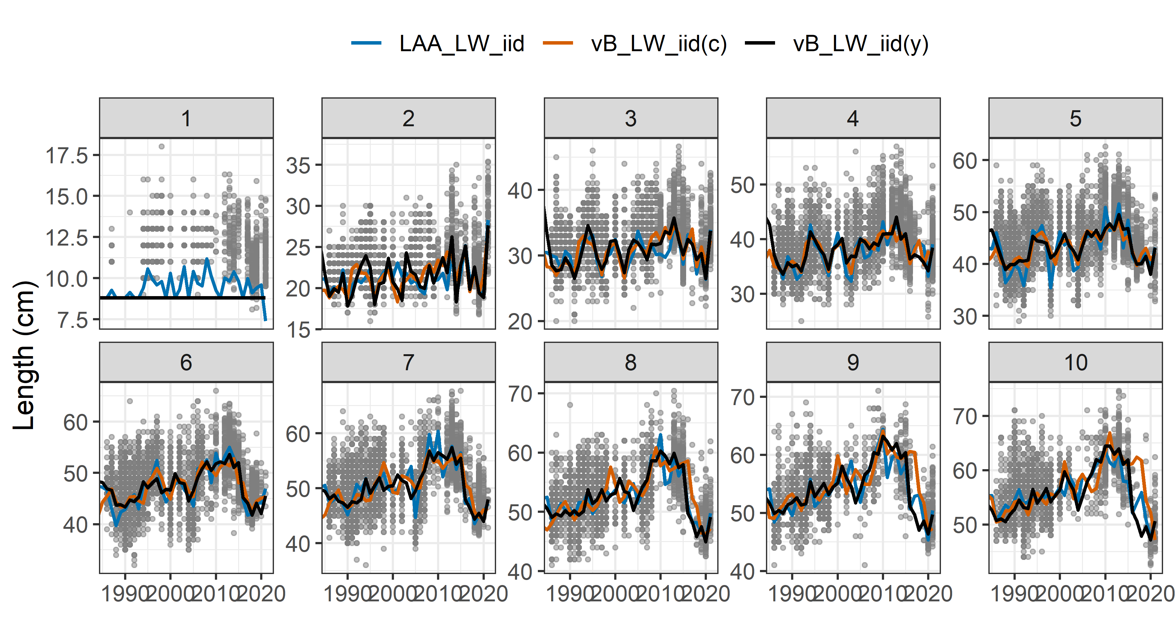
Predicted mean length-at-age (Jan 1st) vs survey observations (\(\sim\) March 1st, not included in the model):
Model comparison
AIC values for models with same input data:
| Model name | (Marginal) AIC | \(\Delta\) AIC |
|---|---|---|
| LAA random effects (\(iid\)) | 827.9 | 0 |
| vB equation (\(iid_y\)) | 4047.2 | 3219.3 |
| vB equation (\(iid_c\)) | 4773.2 | 3945.3 |
| WAA random effects (\(iid\)) | 1188.5 | 360.6 |
Final thoughts
- New tool to explore growth modeling in state-space assessment models
- Non parametric approach seems to outperform a parametric equation
- Non parametric approach is more flexible and deals with fish shrinkage
Future directions (for this project)
- Include survey length information (e.g. marginal length compositions, conditional age-at-length data)
- Add environmental covariate
- Simulation experiment: compare strategies to account for growth variability using WHAM
- Good practices for modeling growth in state-space models
Future directions (in general)
- Software development: include sex, intraannual variability, tagging data, spatial structure
- Comparison among platforms: e.g. SS vs WHAM?
- Ecological research: meaning of all random effects options
Thanks


Cole Monnahan, Jane Sullivan, Jim Thorson, Andre Punt, Tim Miller, Jim Ianelli, Brian Stock
Contact:
gcorrea@uw.edu
giancarlo.correa@noaa.gov
Find more information:
tinyurl.com/wham-growth