Best practices for modeling time-varying growth in state-space stock assessments

Giancarlo M. Correa\(^{1,2}\), Cole Monnahan\(^3\), Jane Sullivan\(^4\), James T. Thorson\(^3\), Andre E. Punt\(^2\)

\(^1\)AZTI, Marine Research, Sukarrieta, Spain. \(^2\)School of Aquatic and Fishery Sciences, University of Washington, Seattle, WA, USA. \(^3\)Alaska Fisheries Science Center, NOAA, Seattle, WA, USA. \(^4\)Alaska Fisheries Science Center, NOAA, Juneau, AK, USA

Somatic growth

Definition: the increase in size or weight of a fish.
In stock assessments: at the stock level.
Growth and recruitment are contributors to the stock biomass.
Time-variable:
- By year, cohort, or age.
- Affected by internal and external factors.

Somatic growth in assessment models

Not explicitly modeled in surplus production models.
Accounted for in VPA and SCAA using empirical weight-at-age.
Explicitly modeled in some integrated models (commonly assumed to be time-invariant).
Ignoring temporal variability may lead to biased results.

State-space models

Process equation: \(E[z_t \mid z_{t-1}] = h(z_{t-1},\theta)\)

Observation equation: \(E[y_t \mid z_t]= g(z_t,\theta)\)

\(\theta\): vector of all unknown model parameters (fixed effects).

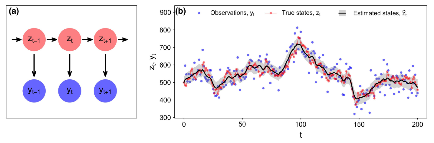
Auger-Méthé et al. (2021)

The Woods Hole Assessment Model (WHAM, Stock and Miller et al. 2021)

Fully state-space age-structured model
Data: catch, indices of abundance, age compositions, empirical weight-at-age, environmental covariates (Ecov)
Separability of total catch and proportions-at-age, as well as annual F and selectivity
Random effects in selectivity, M, NAA, Q, Ecov
Written in TMB and R (user friendly!) ( see R package ).

Growth in state-space models

Goal: implement a flexible framework to model population mean length or weight at age in WHAM.

Data:
- Length compositions
- Conditional age at length (CAAL)
- Ageing error
- Observed mean weight at age

Parameters:
- Population mean length at age (LAA)
- Length-weight (LW) relationship
- Population mean weight at age (WAA)

Growth modeling overview

Correa et al. (2023)

LAA parametric approach

von Bertalanffy (\(k\), \(L_{\infty}\), \(L_{\tilde{a}}\))
Richards (\(k\), \(L_{\infty}\), \(L_{\tilde{a}}\), \(\gamma\))

Length-at-age variability incorporated through two parameters (\(SD_\tilde{a}\) and \(SD_A\)) and a transition matrix (\(\varphi_{y,l,a}\)).

Predicting random effects:

\[log(G_{t}) = \mu_{G} + \delta_{t}\]

\(G\) is a growth parameter, \(t\) represents year or cohort, \(\delta\) are random effects (\(iid\) or \(AR1\) structure).

LAA nonparametric approach

Population mean length at age (\(L_{a}\)) assumed to be fixed effects. \(SD_\tilde{a}\) and \(SD_A\) still needed.

Time variability can be modeled by predicting random effects:

\[log(\hat{L}_{y,a}) = \mu_{L_{a}} + \delta_{y,a}\]

\(\delta_{y,a}\) can be \(iid\), \(2dAR1\), or \(3dGMRF\).

LAA semiparametric approach

Use parametric approach (without random effects) to calculate \(L_{y,a}\).

Predict random effects on \(L_{y,a}\):

\[log(\hat{L}_{y,a}) = \mu_{L_{y,a}} + \delta_{y,a}\]

\(\delta_{y,a}\) can be \(iid\), \(2dAR1\), or \(3dGMRF\).

WAA parametric

Use the LW relationship:

\[w_l = \Omega_1 l^{\Omega_2}\]

Random effects on \(\Omega_1\) and \(\Omega_2\) can also be predicted.

Use transition matrix to calculate population mean weight at age:

\[\hat{w}_{y,a} = \sum_l \varphi_{y,l,a}w_l\]

\(\hat{w}_{y,a}\) can also be fitted to \(\bar{w}_{y,a}\) (observed mean weight at age)

WAA nonparametric

Like the LAA nonparametric. Population mean length at age (\(w_{a}\)) assumed to be fixed effects.

Time variability can be modeled by predicting random effects:

\[log(\hat{w}_{y,a}) = \mu_{w_{a}} + \delta_{y,a}\]

\(\delta_{y,a}\) can be \(iid\), \(2dAR1\), or \(3dGMRF\).

More new features

Selectivity

Originally, only selectivity-at-age functions were available.

New functions added:

Age double normal (6 parameters).
Length logistic (2 parameters).
Length decreasing logistic (2 parameters).
Length double normal (6 parameters).

More new features

Environmental covariates

New growth-related parameters can be linked to an environmental covariate. For example:

\[P_t = P exp(\beta_1 X_t)\]

\(P\) is the base state (parameter) value. Other links are also available (polynomials). Lags can be modeled.

Applications

Methods applied to three stocks in Alaska:

Gulf of Alaska Walleye pollock: age data, observed mean weight at age, WAA nonparametric.
Gulf of Alaska Pacific cod: length and CAAL data, LAA parametric.
Eastern Bering Sea Pacific cod: length data, LAA parametric with time-varying \(L_\tilde{a}\).

See Correa et al. (2023) Modeling time-varying growth in state-space stock assessments. ICES Journal of Marine Sciences.

Good practices

Strategies that have been shown through research and evaluation to be effective and/or efficient, and to reliably lead to a desired result.

Simulation experiment

Goal: provide guidelines for growth modeling in state-space assessment models under diverse scenarios.

Data type: age compositions vs length compositions vs CAAL (random vs stratified sampling).
Data source: fishery vs survey.
Data quality: data rich vs data poor.
Modeling approach: parametric vs nonparametric vs semiparametric vs Ecov.
Time-varying parameter: changes in \(k\), \(L_{\infty}\) or \(L_{\tilde{a}}\).

Simulation experiment

Methodology:

Operating model: simulates the true population dynamics. Changes in growth by varying \(k\), \(L_{\infty}\) or \(L_{\tilde{a}}\).
Sample data from operating model.
Estimation model uses sampled data with assumptions on the population dynamics.

Preliminary results

Conclusions

Expansion of the applicability of state-space assessment models.
Implementation of a flexible framework to model time-varying growth in state-space assessment models.
Recommendations to model time-varying growth under diverse scenarios.

Thanks

Tim Miller, Brian Stock, Jim Ianelli, Steve Barbeaux, Peter Hulson

Contact:
gmoron@azti.es

Find more information:
tinyurl.com/wham-growth