Responding to climate-driven changes in growth in the modern stock assessment models
Giancarlo M. Correa\(^1\), Cole Monnahan\(^2\), Jane Sullivan\(^3\), James T. Thorson\(^2\), Andre E. Punt\(^1\)
\(^1\)University of Washington, Seattle, WA
\(^2\)Alaska Fisheries Science Center, NOAA, Seattle, WA
\(^3\)Alaska Fisheries Science Center, NOAA, Juneau, AK
Growth modeling in state-space models
Growth modeling overview
In the population:
Mean length-at-age (LAA)
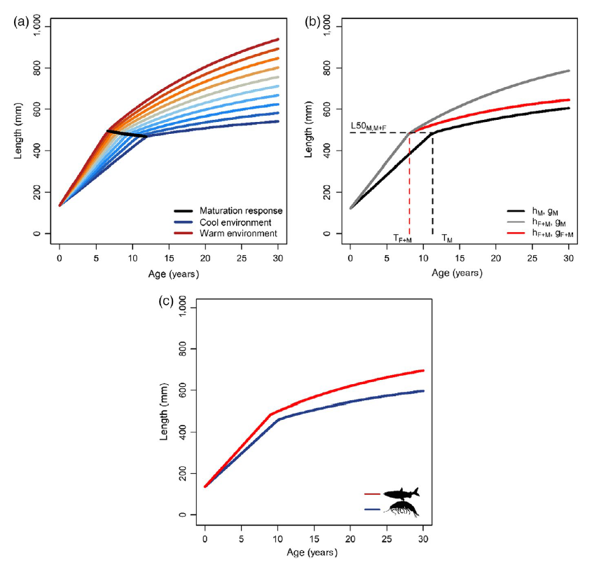
Growth equation (von Bertalanffy)
The mean length-at-age at the start of the year (\(y=1\)):
\[\tilde{L}_{y,a} = L_{\infty}+(L_1 - L_{\infty})exp(-k(a-1))\]
\(a=1\) is first age in WHAM. Then, when \(y>1\):
\[\tilde{L}_{y,a} = \begin{cases} L_1, & \mbox{if } a=1 \\ \tilde{L}_{y-1,a-1}+(\tilde{L}_{y-1,a-1}-L_{\infty})(exp(-k)-1) & \mbox{otherwise} \end{cases}\]
Mean length-at-age (LAA)
Growth equation (von Bertalanffy)
Then, to calculate the mean length-at-age at any fraction of the year:
\[L_{y,a} = \tilde{L}_{y,a} + (\tilde{L}_{y,a} - L_{\infty})(exp(-kf_y)-1)\] \(f_y\) is the year fraction.
Mean length-at-age (LAA)
Growth equation (von Bertalanffy)
Random effects on growth parameters can be predicted (notice log scale):
\[log(L_{\infty_t}) = \mu_{L_\infty} + \delta_{1,t}\]
\[log(k_t) = \mu_{k} + \delta_{2,t}\]
\[log(L_{1_t}) = \mu_{L_1} + \delta_{3,t}\]
\(t\) represents year or cohort effects and can be \(iid\) or \(AR1\).
Mean length-at-age (LAA)
LAA random effects
For this case, mean length-at-age ( \(\mu_{\tilde{L}_{a}}\), notice log scale ) are assumed to be parameters and can be estimated. \(\sigma_{y,a}\) still needed.
Time variability can be modeled by predicting random effects:
\[log(\tilde{L}_{y,a}) = \mu_{\tilde{L}_{a}} + \delta_{y,a}\]
\(\delta_{y,a}\) can be \(iid\) or \(2dAR1\) (full variance-covariance matrix).
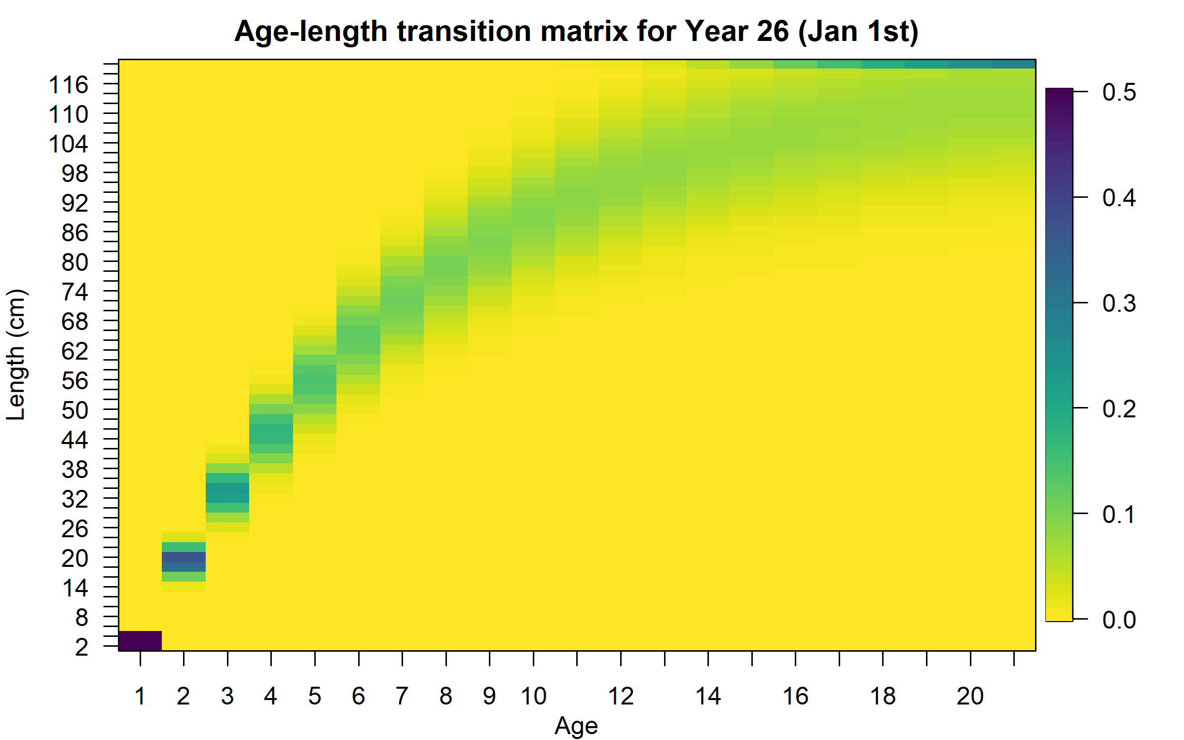
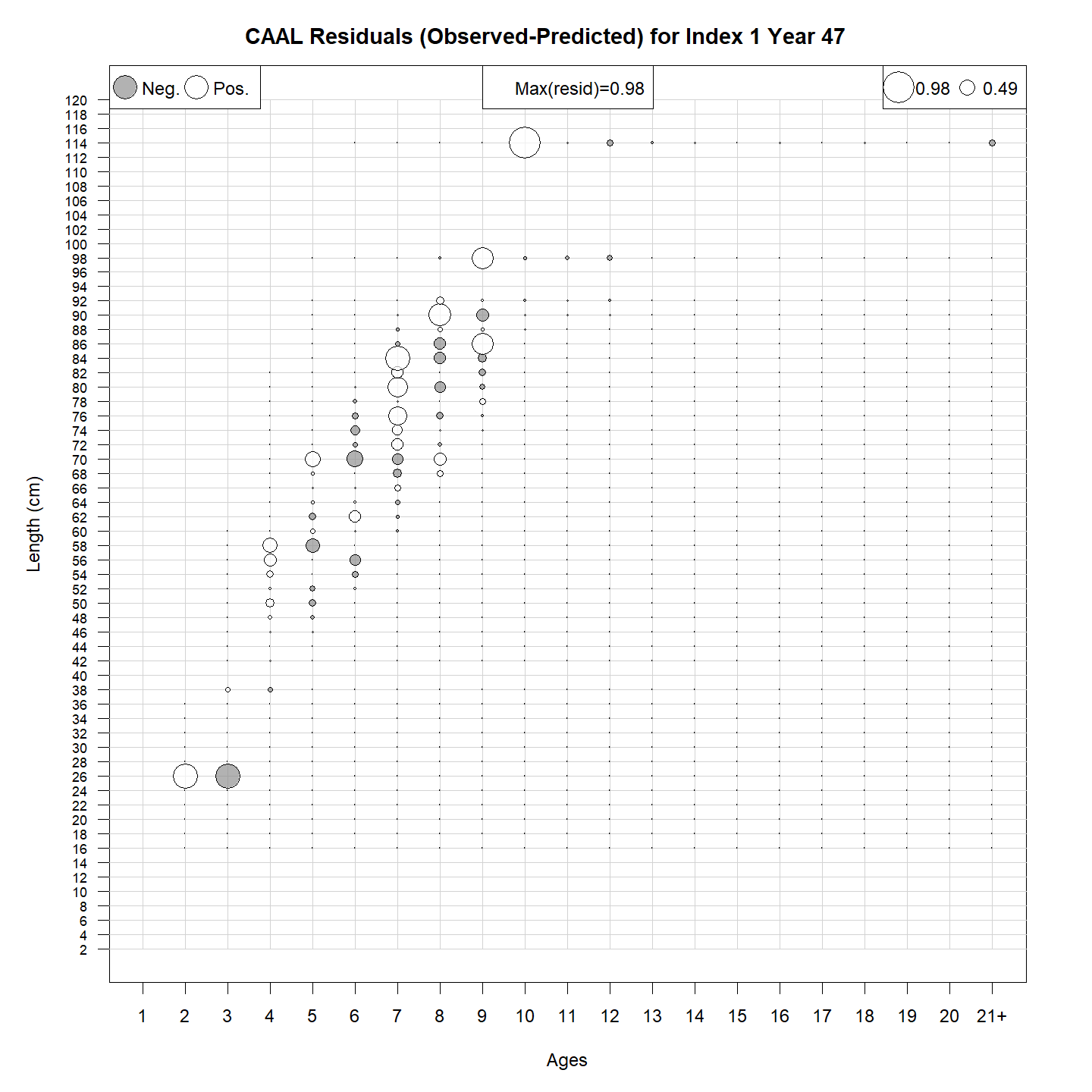
Age-length transition matrix
Also, \(L_{y,a}\) and variation of length-at-age ( \(\sigma_{y,a}\) ) are used to calculate the age-length transition matrix (Stock Synthesis - SS - approach):
\[\varphi_{y,l,a} = \begin{cases} \Phi(\frac{L'_{min}-L_{y,a}}{\sigma_{y,a}}) & \mbox{for } l=1 \\ \Phi(\frac{L'_{l+1} - L_{y,a}}{\sigma_{y,a}}) - \Phi(\frac{L'_{l} - L_{y,a}}{\sigma_{y,a}}) & \mbox{for } 1<l<n_L \\ 1-\Phi(\frac{L'_{max} - L_{y,a}}{\sigma_{y,a}}) & \mbox{for } l = n_L \end{cases}\]
Where \(\Phi\) is standard normal cumulative density function, \(L'_{l}\) is the lower limit of length bin \(l\), \(L'_{min}\) is the upper limit of the smallest length bin, \(L'_{max}\) is the lower limit of the largest length bin, and \(n_L\) is the largest length bin index.
Age-length transition matrix
![]()
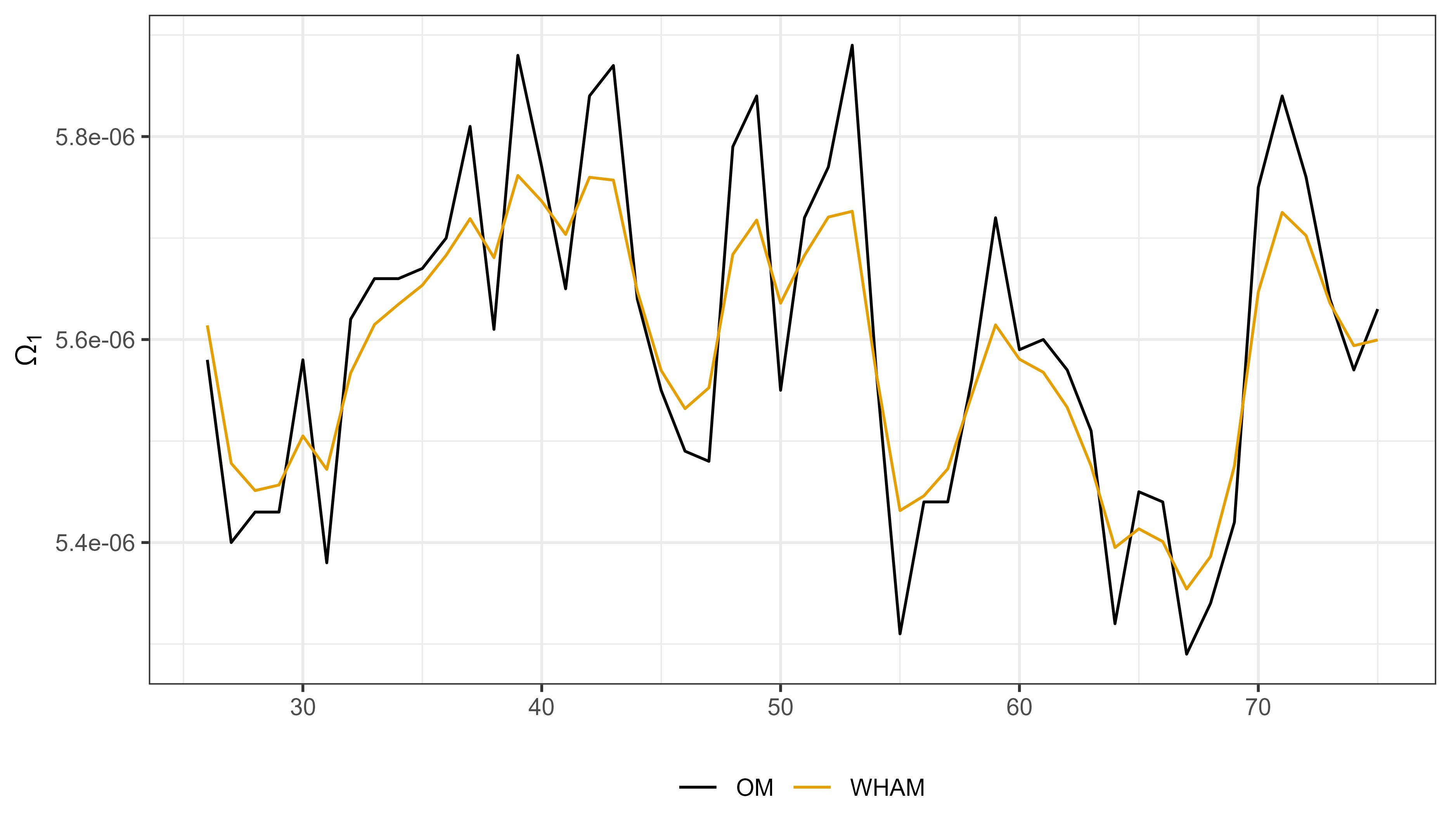
Mean weight-at-age (WAA)
Length-weight relationship
Optional when empirical weight-at-age not provided:
\[w_l = \Omega_1 l^{\Omega_2}\]
Random effects on \(\Omega_1\) and \(\Omega_2\) can also be predicted.
Then:
\[\hat{w}_{y,a} = \sum_l \varphi_{y,l,a}w_l\]
\(\hat{w}_{y,a}\) can also be fitted to \(w_{y,a}\) (observed mean weight-at-age)
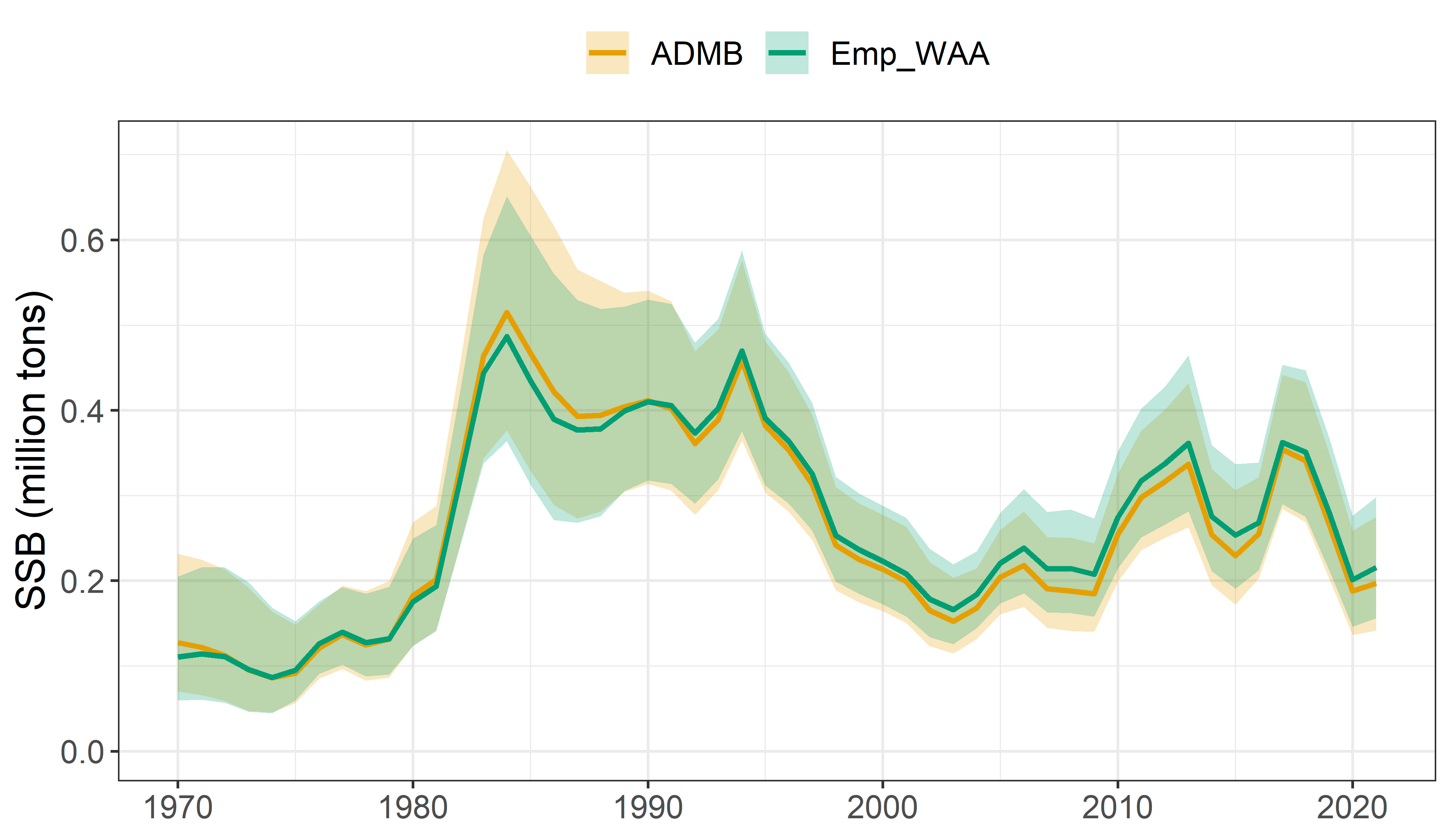
Mean weight-at-age (WAA)
WAA random effects
Like the LAA random effects. Mean weight-at-age ( \(\mu_{\tilde{W}_{a}}\), notice log scale ) are assumed to be parameters and can be estimated.
Time variability can be modeled by predicting random effects:
\[log(\tilde{W}_{y,a}) = \mu_{\tilde{W}_{a}} + \delta_{y,a}\]
\(\delta_{y,a}\) can be \(iid\) or \(2dAR1\) (full variance-covariance matrix).
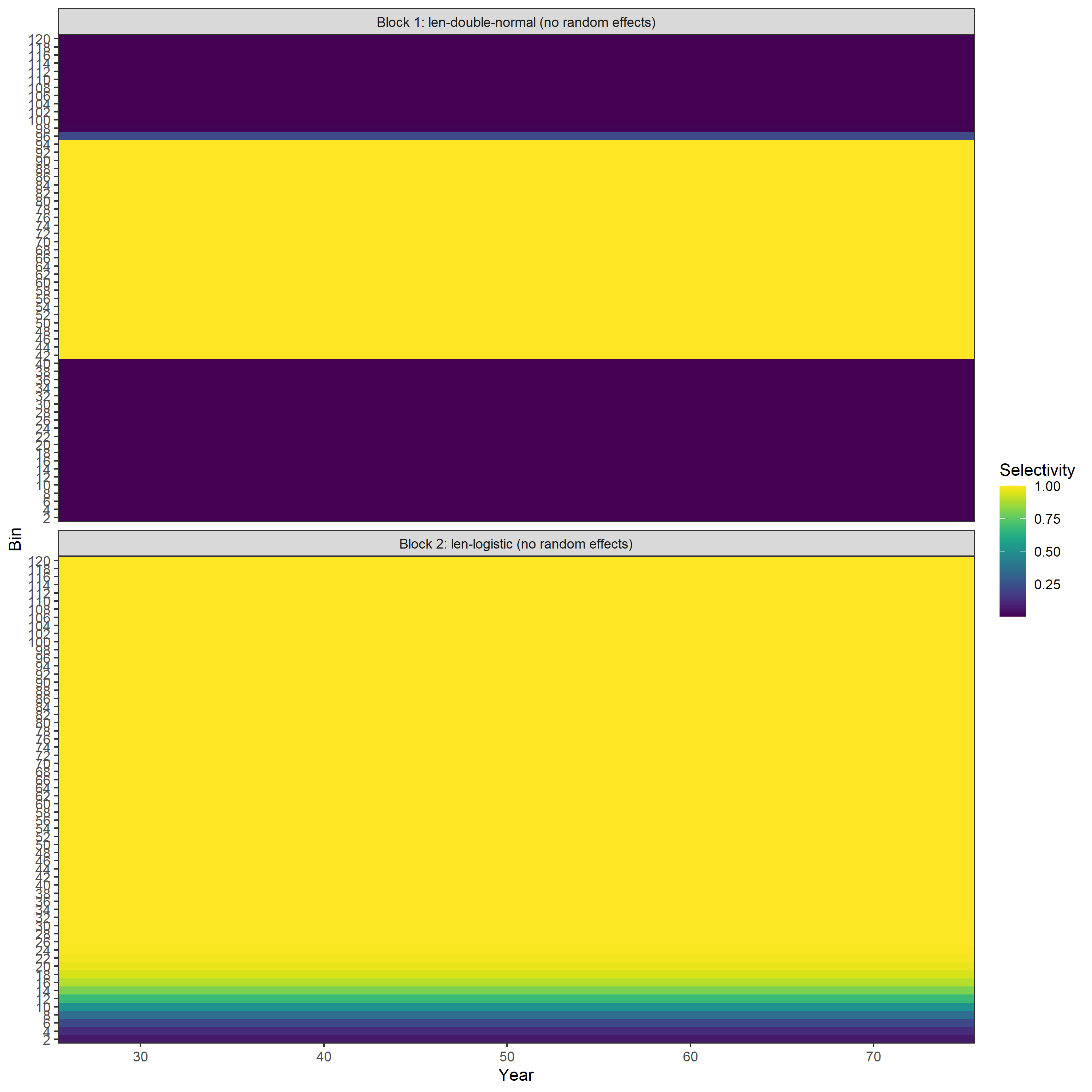
Selectivity
Originally, only selectivity-at-age functions were available (age-specific, logistic, double-logistic, decreasing-logistic)
New functions added:
double-normal: by age. SS-like (Methot and Wetzel, 2013)
len-logistic: increasing logistic at length
len-decreasing-logistic: by length
len-double-normal: by length
Environmental covariates
WHAM separates process (random walk or AR) and observation error for environmental covariates.
An environmental covariate can be linked to a state (i.e. parameter):
\[P_t = P exp(\beta_1 X_t)\]
\(P\) is the base state (parameter) value. Other links are also available (polynomials). Lags can be modeled.
 Morais and Bellwood (2020)